A* Pathfinding in Video Games

Pathfinding has a long tradition in video games. Whenever a character wants to move from one point to another, some way of evaluating how to do that without colliding with the environment is needed. This is where pathfinding comes in. The following post looks at using the A* algorithm for geographic pathfinding.

Developers use the A* search algorithm to find the cheapest path from one point to another in a pathfinding problem. In the domain of geographic pathfinding for games, this algorithm is one of the most popular, because it offers great efficiency relative to its low complexity. That said, with a very high number of agents, it can still cause CPU performance problems.

One necessary precondition is that the game world is divided into a grid of points. This grid can be two- or three-dimensional. In either case, the size of the grid cells should be chosen carefully and, if necessary, simplified relative to the game world. In a large, procedurally generated game world with a high level of detail, where units can occupy continuous coordinates, the search space for a heuristic search would be too performance-heavy. Accordingly, games that use a simplified, rasterized game world are best suited to A* pathfinding.

In this case, objects block discrete grid points: an object either blocks the grid point or it doesn't. Starting at a point A, the algorithm examines the eight grid points neighboring A (referred to as nodes) based on their cost of reaching the target node B.

f(x) = g(x) + h(x)

A metric f(x) is used to calculate the cost. For node x, g(x) describes the sum of the costs to reach that node, and h(x) is the estimated cost to reach the goal from there. Horizontal and vertical movement is typically weighted at 10, and diagonal movement at 14. These weights originate from the Pythagorean theorem.

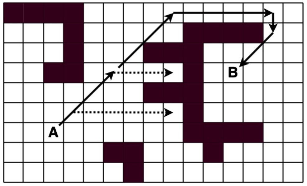
If you number all of A's neighbors clockwise starting with the neighbor above as x0, the cost of node x1 (located to the upper right of A) would come out as follows:

f(x1) = (14) + (14 ∗ 3 + 10 ∗ 6) = 116

Node x6 would produce the following result:

f(x6) = (10) + (14 ∗ 3 + 10 ∗ 7) = 122

The node with the lowest result is chosen as the central node for the next iteration, and its neighbors are examined in the following step. Nodes considered obstacles are ignored during evaluation. In addition to calculating the cost, the node whose neighbors are being examined is referenced within node x. Ideally, this reference is later used to trace back the optimal path that was found. During the iterations, the algorithm maintains two lists of nodes — the open list and the closed list. All examined nodes are added to the open list. Before the first iteration, only the starting node is in the open list. After the first iteration, all walkable neighbors of the starting node are in the open list. All nodes whose neighbors have already been examined are stored in the closed list. That's why, after the first iteration, the starting node is in the closed list.

In the second iteration, the algorithm picks the cheapest node from the open list and starts over from the beginning, examining that node's neighboring cells for their cost. Because an overarching list of all examined nodes is always maintained, the algorithm is able to maneuver its way out of dead ends, as shown in the figure. When the last node in a dead end is examined and added to the closed list, other, previously bypassed nodes are still available.

The algorithm ends when the open list is empty or the examined node is the target node. In the first case, all reachable nodes would have been examined and added to the closed list. In that case, there is no solution — the target point is unreachable. But if the target node is reached, you can trace back from it via each node's predecessor reference all the way to the starting node. This produces a list of nodes describing the optimal path to the goal. In that case, the algorithm was successful.

A useful extension of the A* pathfinding algorithm is influence maps. These are simply an additional layer, another grid that gets updated at runtime. Accordingly, such functionality is implemented with memory and performance efficiency in mind. An influence map can, for example, be used to track which nodes are visible to players or not. Another use case is tracking which cells lie within the attack range of enemy units. These values can be factored into the cost calculation at every iteration.